Factor Analysis

Uses

• classify or reduce data by summarizing a large number of variables with a smaller number of "derived" variables
• explore and structure a content area by determining the number of indepedent dimensions required to represent a set of variables
• map unknown concepts by identifying underlying constructs (i.e., factors) that explain correlations among sets of variables

Assumptions

• The underlying data must be distributed multivariate normally and relationships must be linear. If such requirements are not met, multi-dimensional scaling may be an alternative.
• The number of data points should be the greater of either N=100 or N=5 x the number of raw data variables used.
• Examine whether data contain sufficient correlations to warrant PCA by testing with Bartlett's sphericity test (i.e., whether the correlation matrix (variance/covariance matrix) is an identity matrix), or Kaiser-Meyer-Olkin Measure of Sampling Adequacy indicates the proportion of variance in your variables which is shared among variables. With KMO between 0.5 and 1, a factor analysis may be of value.
• Matrix Ill-Conditioning: Ill-conditioned matrices produce estimated coefficients that are are unstable (i.e. small changes within the range of measuring error of the variables can lead to disproportionately large changes in the estimates)

How this is done

Each item is defined by its value on a series of measured variables, where a priori each variable is viewed as being independent or orthogonal from the others. Factor analysis in a way rearranges the coordinate system that defines these items in order to more accurately reflect the situation where some variables may actually correlate with each other. Correlations exist because the variables to some degree measure the same thing. For instance if we measure body length, body width, and body depth of a series of individuals we won't be greatly surprised if we find that these correlate. The goal of factor analysis is to properly account for such correlations and to thereby identify those underlying factors which may explain them. New axes are constructed as linear combinations of the underlying variables. It is possible for us to extract the same number of axes as there are original variables.

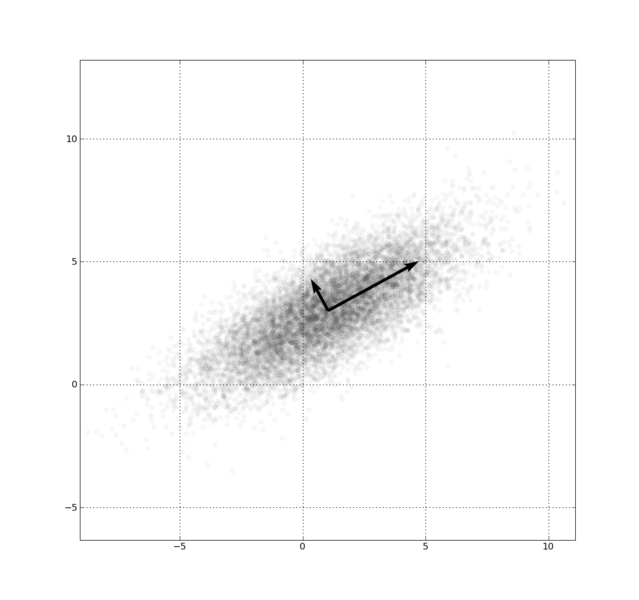
Fig. 1., PCA of a multivariate Gaussian distribution centered at (1,3) with a standard deviation of 3 in roughly the (0.878, 0.478) direction and of 1 in the orthogonal direction.

The Correlation matrix contains information about the degree to which information in different variables overlaps. As it represents a standardized variance/covariance matrix, each variable has equivalent representation in the overall picture. The Total variance contained within a dataset of n orthogonal, standardized variables (each with s = 1) is always n*1. Rank: the number of components contributing to the variance. A data matrix may be rank-deficient in the presence of excessive (perfect) correlations among the original variables. This occurs when different variables are not linearly independent of each other (e.g., one variable is the straight sum of two other variables). In this case an inverse of the matrix cannot be formed for an extraction of eigenvectors. Variables are by definition considered orthogonal. When PCA is performed on the correlation matrix, standardized variances are the base of the explanation, when PCA is performed on the variance/covariance matrix unstandardized measures are used.

Principal Components Analysis (PCA) is one form of factor analysis. It allows us to extract linear combinations of the original variables. This technique uses Eigenvalue Decomposition where 2 matrices are extracted from the n x n correlation matrix. Using a series of complex linear algebraic techniques, such as Singular Value Decomposition, a set of component matrices is extracted to satisfy the following relationship

DataMatrix = U * S²* U'.

Axes are specified by these two matrices, where the Eigenvector Matrix (U) contains information about the orientation of a series of extracted axis in our original data space, while the Eigenvalue Matrix (S²) measures each axis' size.

Eigenvector Scores (U) are orthonormal and describe the axis' direction. Eigenvectors are always at right angles to each other (orthogonal) and are normalized to unit length of 1 (i.e., the squares of the elements in each eigenvector always sum to 1). The orthogonal nature of eigenvectors can be confirmed by examining their crossproducts (i.e., always zero as the cosine of 90^o is always zero). The Eigenvector Matrix is also its own transposed inverse (U'). Thus multiplying the Eigenvector score matrix with its transposed form will produce the identity matrix (I). U * U' = I. The eigenvector matrix contains the standardized regression coefficients (i.e., slopes) for a multiple linear regression equation in wich the original variables are used to explain each principal axis.

The Eigenvalue matrix (S²) describes the magnitude of each eigenvector's size along the diagonal of the matrix, and is measured in variance units. Each eigenvalue can thus also be expressed in relative form as % of total Variance explained by each PC axis. The square root of the Eigenvalues produces the Singular Value Matrix (S), and, like the standard deviation, it describes the true magnitude of the eigenvectors in units defined by the data space.

Matrix of Factor Loadings (i.e., component loadings, factor pattern matrix) characterizes the actual eigenvectors in true size (U*S) as they combine both information of magnitude (its singular value) and direction (its unit-length eigenvector matrix). Factor loadings are also the correlation coefficients (r) between the original variables and the factors.

Matrix of Squared Factor Loadings (U*S)² expresses the percentage of variance in each variable explained by each factor (r²). The sum of the squared factor loadings for each Eigenvector adds up to the eigenvalue.

Factor Scores: Recast the data points into new axes: Use the matrix of factor loadings to obtain scores (i.e., new coordinates) for each datapoint. The sum of squared scores on a variable will add up to n-1 where n is the number of data elements. The sum of the squares of the columns of the factor score matrix is the inverse of the eigenvalue corresponding to that column.

Factor analysis does, however, not tell us how many different factors (i.e., independent axes) may be extracted in a meaningful way. Biological reasoning should provide us with arguments about how many different underlying constructs should be present. Alternatively, based on measures of variance explained by each successive axis, we may use different criteria for whether a particular axis still contains meaningful information.

• Kaiser Criterion: We extract values with eigenvalues > 1 (i.e., the extracted variable explains more than each intial variable did going into this analysis)
• Scree Test: We graph eigenvalues of successive axes to determine the area of the graph where the line plot levels off. It is ok to choose the solution with the most appealing factor structure.

Communality: the proportion of a variable's variance that is explained by a factor structure. A communality is denoted by h2. See communality measures for each original variable the proportion of its variance that it shares with other variables, i.e., variance which can be represented by communal factors; sum of the squared factor loadings for a given variable across all included factors; 1.0, or 100% if no factors are dropped. The proportion of variance that is unique to each item is the variables' total variance minus the communality

• Use multiple regression techniques to regress variables on the coordinates in different dimensions (PC scores). Complex variables are those that load on two or more factors.
• Factor rotation simplifies the factor structure for interpretation. A structure becomes simpler when the number of zeros or near-zero entries in the factor matrix increases.The actual orientation of axes in the final solution is arbitrary. For example, one can rotate a map, yet the distances between locations on it remain the same. You can rotate the factor space for improved interpretation by minimizing the number of variables with high loadings on each axis.